Government Finance (1)

Illustrating Steve Keen's Substack post

Steve Keen recently completed a book called Rebuilding Economics from the Top Down, and has published chapter 11, about the “mixed credit-fiat monetary system” on his Substack. Here I’m going to translate the Godley Tables¹ from that article into the One Lesson’s arrow notation for transfers of raw net worth². I’ll discuss the interpretation on another occasion.

It might seem a little dry, but do check each of the diagrams to make sure you understand what’s going on, and take time to appreciate the intuitive representation of the diagrams.

We’ve already seen the types of transaction which Keen discusses — in the series on the circular flow of income, but here I’ll follow the structure of his article.

The sectors which Keen uses are:

1. Treasury. The part of government which manages all the government’s spending and taxation.

2. Central bank. E.g. the Fed or the Bank of England.

3. Banks. All other banks.

4. NBPS. Non-bank private sector i.e. everyone else: mainly households and non-bank firms.

The fundamental accounting for Credit Money

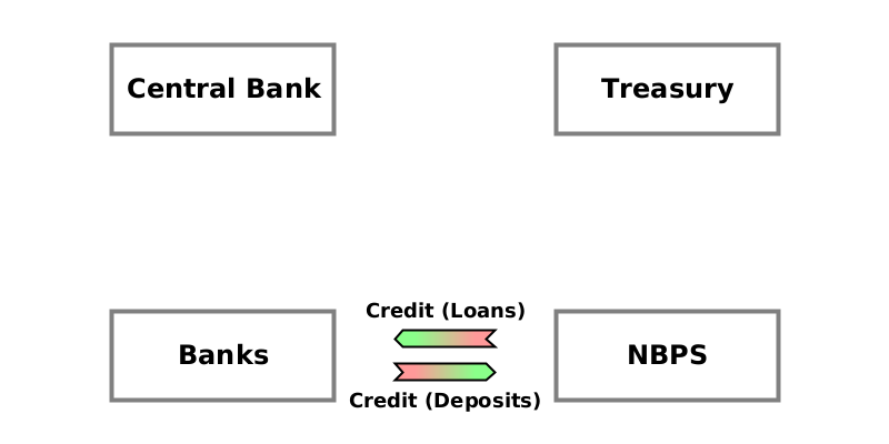
Keen’s Figure 37 shows banks creating credit money (“deposits”) by lending. This should be very familiar by now. The banks create new debts owed to the NBPS (deposits) and the NBPS creates new debts owed to the banks (loans).

This shows the main flows, but excludes some which can be very important:

• Interest (a pink-to-green arrow from NBPS to Banks)

• Defaults by borrowers (a green-to-pink arrow from Banks to NBPS)

• Running costs, such as wages, building maintenance, heating and lighting, consumables, etc. (a pink-to-green arrow from Banks to NBPS, and services or goods, subsequently consumed, in return)

• Dividend payments (a pink-to-green arrow from Banks to NBPS, and a green-to-pink arrow).

Each of these leads to an equal and opposite change to banks’ equity.

Defaults in particular can have a profound effect if bad debts accumulate.

Government spending and taxation

Keen’s discussion of government involvement starts with analysing government spending and taxation separately, but doesn’t complete all the Godley tables for all sectors. Instead, it combines spending and taxation into a single flow called deficit (spending minus taxation). Here I’ll show the full diagrams for spending and taxation separately first, then show how to combine them to follow Keen’s approach of treating them as a single ‘deficit’ flow.

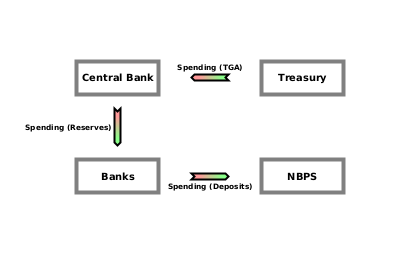
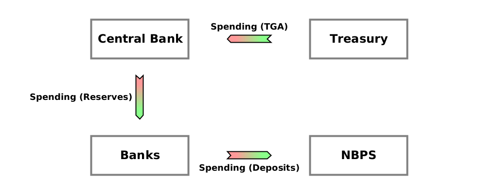
TGA means the Treasury General Account — the Treasury’s bank account at the central bank³. “Spending” represents the amount spent (say over a year). It:

1. Decreases the Treasury’s assets and decreases the central bank’s liabilities. (The Treasury is giving up some of its TGA balance.

2. Increases the central bank’s liabilities and increases the banks’ assets. (The central bank is creating new reserves in the banks’ accounts).

3. Increases the banks’ liabilities and increases the NBPS’s assets. (The banks are creating new deposits in NBPS accounts).

The overall effect is to transfer some of the Treasury’s RNW to the NBPS. The central bank and the other banks have their RNW both increase and decrease by the same amount, so their RNWs are unchanged.

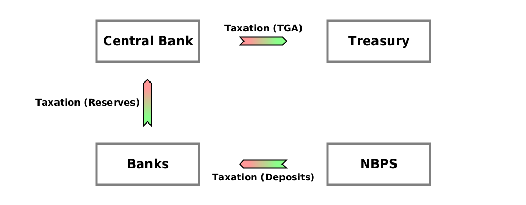
Taxation works exactly in reverse.

Again, the banks and central bank each have their RNW both increase and decrease by the same amount, so their RNWs are unchanged. The overall effect is a transfer of NBPS’s RNW to the Treasury.

Combining spending and taxation

When we combine government spending and taxation into a single deficit flow (government spending minus taxation), the diagram for the overall result will depend on whether spending or taxation is higher. If spending is higher, the result will be like the government spending diagram (with a RNW transfer from Treasury to NBPS) — just replace “Spending” with “Deficit”. (This is equivalent to Keen’s Figure 46). And if taxation is higher, the result will be like the taxation diagram (with a RNW transfer from NBPS to Treasury) — just replace “Taxation” with “Surplus” (the opposite of deficit).

Government bonds

The next section discusses how government bond⁴ sales to the central bank, other banks, or the non-bank private sector work (or would if they happened — central banks are usually not allowed to buy government bonds directly from the government).

Central bank buys bonds

If the government starts with an empty TGA, and runs a deficit (spending more than it receives in taxes), the TGA balance becomes negative, which is a bit ugly. Keen examines in his Figure 47 how this could be avoided if the government issued new bonds to the central bank directly. (If the subscripts and superscripts look scary, you don’t need to worry. “Bond” with subscript “T” and superscript “CB” just means the dollar⁵ amount of bonds issued by the Treasury and bought by the Central Bank. “Bonds[CB]” just refers to the account in which the bonds are recorded at the central bank).

This is a normal borrowing arrangement. Two new debts are created. The debt owed by the central bank to the Treasury (top arrow) increases the balance in the TGA, so it needn’t be negative. In exchange, the Treasury gives a bond to the central bank.

Since both new debts are equal, there isn’t really much happening here. It’s just placing entries in different accounts to leave the TGA account with a non-negative balance.

Interest payments on bonds would become profits of the central bank. But since central banks remit their profits to the Treasury, Keen quite reasonably leaves out this detail.

Other banks buy bonds

Private sector banks often buy government bonds. To do this, a bank transfers some of its reserves at the central bank to the TGA, and it receives the bond in exchange. This is shown in the Godley Tables of Figure 49. (“Bond” with subscript “T” and superscript “B” just means the dollar amount of bonds issued by the Treasury to the banks. “Bonds[B]” just refers to the accounts in which the bonds are recorded at the banks).

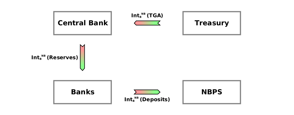
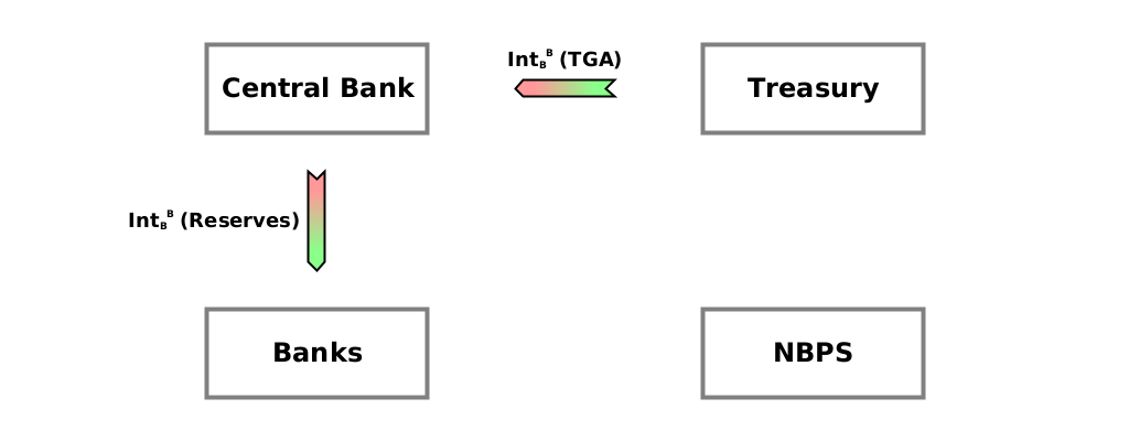
The holder of a government bond receives interest payments from the Treasury. When the holder is a bank with an account at this central bank, this is as simple as the Treasury transferring some of its balance in the TGA to the reserve account of the bank, as also shown in Keen’s Figure 49. (“Int” with subscript “B” and superscript “B” just means the dollar amount of interest paid by the Treasury on the bonds to the banks — by making a transfer from the TGA to the accounts of the banks at the central bank).

Non-bank buys bonds (from banks)

Non-banks can also buy government bonds. Typically they don’t buy them directly from the Treasury, but buy them from banks who have previously bought them from the Treasury.

In his Figure 50, Keen shows the transfer of the bond from banks to the non-bank private sector as a write-off of the original debt and the creation of a new debt, rather than simply the transfer of an existing debt asset from the banks directly to the non-bank private sector. This doesn’t really make a difference — the result is the same. (“Bond” with subscript “T” and superscript “NB” just means the dollar amount of bonds issued by the Treasury to the banks. “Bonds[NB]” just refers to the accounts in which the bonds are recorded in the non-bank private sector).

Finally, also in Figure 50, Keen shows interest payments to the non-bank private sector due to their holdings of government bonds. (“Int” with subscript “B” and superscript “NB” just means the dollar amount of interest paid by the Treasury on the bonds to the non-banks — by making a transfer from the TGA to the accounts of the banks at the central bank).

This is very similar to the payment of interest to banks, except that there’s one extra step in the indirect payment: the banks create deposits for the holders of the bonds in the non-bank private sector. Notice the similarity to government spending above.

Summary

There isn’t really anything here which we haven’t seen before, but this particular arrangement of diagrams is going to be useful because next time I’m going to discuss what I think is a serious problem with Keen’s analysis. It’s also a problem at the heart of MMT⁶, so I expect that will be my most controversial post so far. I’m already looking forward to the feedback…

Thanks for reading!

1. A Godley Table represents a balance sheet, and shows both its starting point (at the beginning of a simulation), and a set of transactions which can cause it to change over time.

2. Someone’s raw net worth (RNW) is what they own plus what they’re owed minus what they owe. It is a “heterogeneous” sum/difference, which just means that things of different types are added and subtracted, not monetary “values” which have been assigned to them.

3. This is the term used in the USA. The UK government’s main account with the Bank of England is called the Consolidated Fund (CF).

4. A bond is just a promise to repay the amount borrowed after a certain amount of time, as well as promises to pay interest in the meantime, perhaps at 6-monthly intervals. It’s basically a small collection of debts.

5. Or other currency as appropriate.

6. Modern Monetary Theory — a theory of economics which claims to be a neutral description of government accounting, but which I’ll be challenging based on an analysis of raw net worth.